
Main task: reporting clinical trials
Purpose of regulatory submissions is to show efficacy and safety of new drugs.
- Deliver analysis reports, datasets, and software
- Health Authorities (HA) need to be able to reproduce key results
Davide Garolini & Leena Khatri
This material is based on the original work from the {gtreg} workshop by Shannon Pileggi and Daniel Sjoberg, available here, and adapted under a Creative Commons Attribution 4.0 International License.
| Time | Activity |
|---|---|
| 09:00 - 09:20 | Why Change? |
| 09:20 - 10:10 | Getting there (P1) |
| 10:10 - 10:20 | Break |
| 10:20 - 11:10 | Getting there (P2) |
| 11:10 - 11:20 | What do we expect? |
| 11:20 - 11:30 | Additional resources: Collaborate! |
Please add any questions to the public Zoom chat. These may be answered in the moment or addressed at the end depending on context.
Purpose of regulatory submissions is to show efficacy and safety of new drugs.
Benefits for all
Cost Efficiency: R is free, reducing software costs.
Flexibility: R offers greater customization and a vast package ecosystem.
Community Support and Collaboration: R has a large, active community driving rapid innovation.


What’s in it for us
2017 → PoCs
{rtables}, {teal} for interactive work were launched and presented at RinPharma
2021 → Open-source
{rtables} made the first CRAN release, followed by open source of the codebase to kick off collaborations with other companies
2023 → Adoption of tools and systems
Validated environment to deliver our vision of R in submissions
2024 → E2E submission in R
→ Regulatory Acceptance: R is increasingly accepted by regulatory agencies.
Evolution or Revolution?
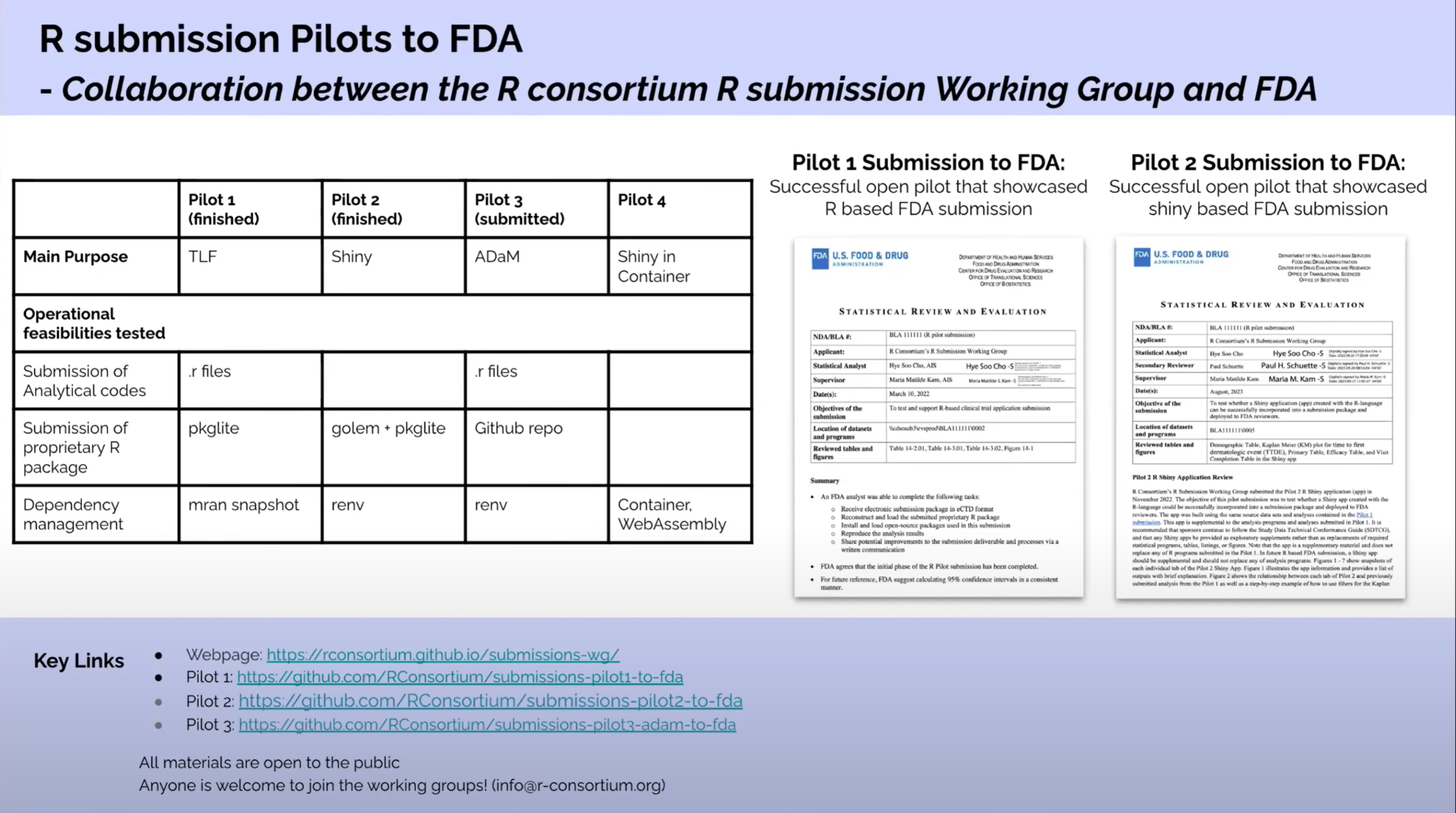
1.-2. Docker or WebAssembly (Pilot 4) 3. Even if p-hacking is NOT technology dependent, the ease-of-use and tweaking binds interactive features to the exploratory world
From Hye Soo Cho, FDA, in R/Adoption Series: R and Shiny in Regulatory Submissions
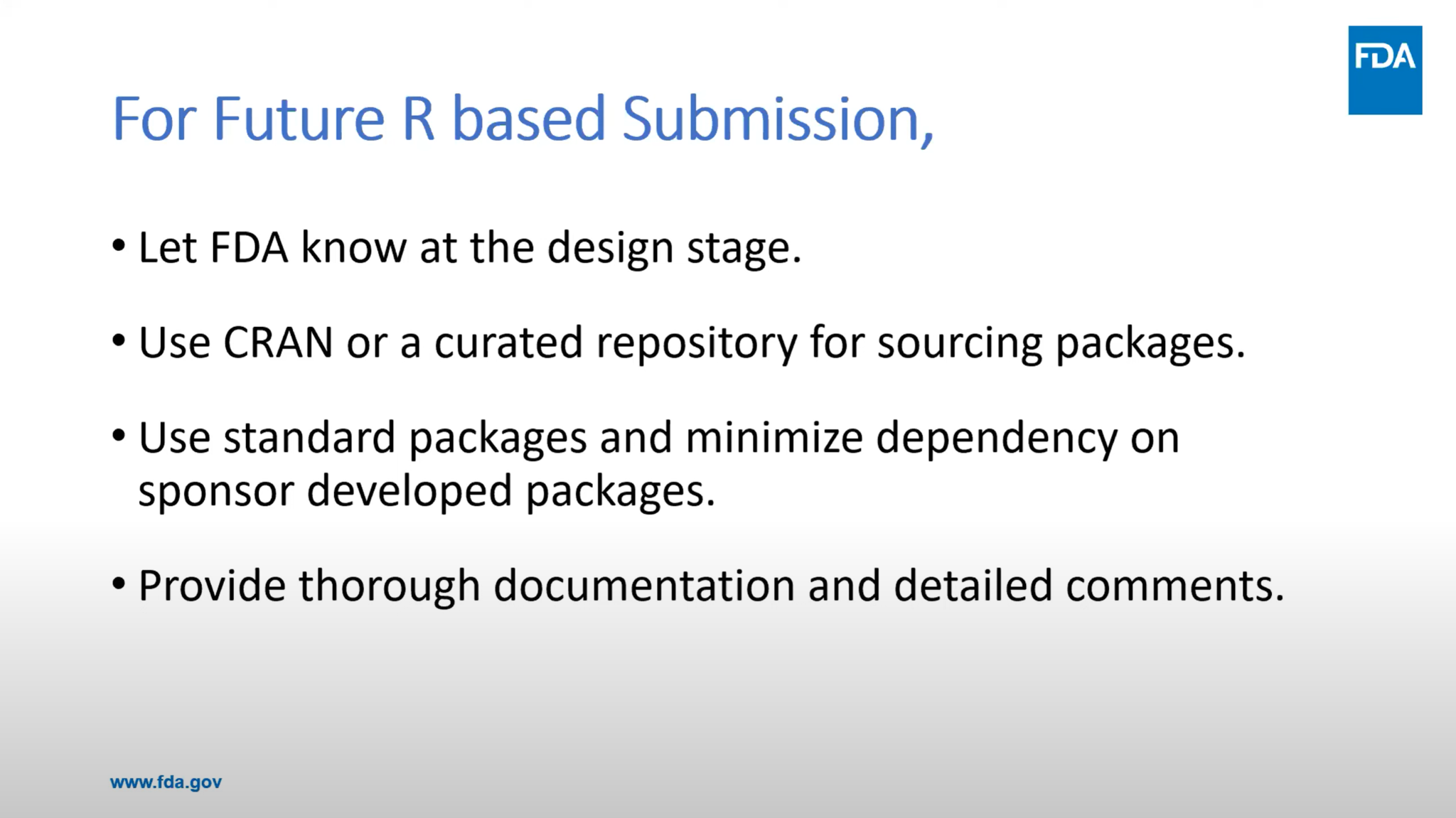
Reproducibility and validation - CRAN and extensive CI/CD testing, precise documentation and versioning
Open-source - Collaboration and transparency accelerates industry towards standardization due to a wider adoption (faster submissions?)
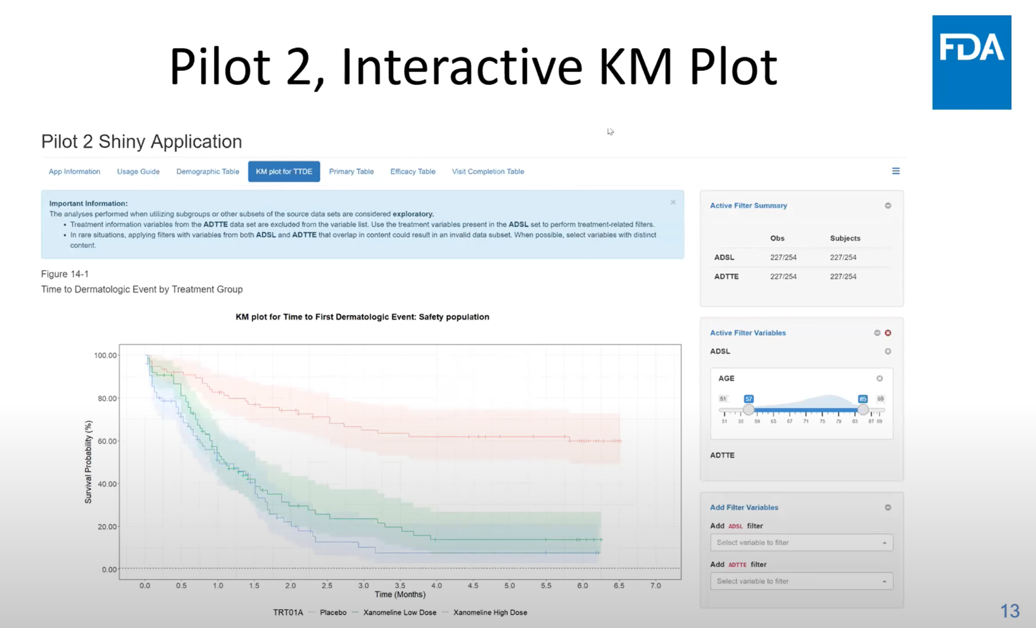
Interactivity - {teal} as exploratory tool, integrates standard TLF, enables novel findings, and fast reviewer responses
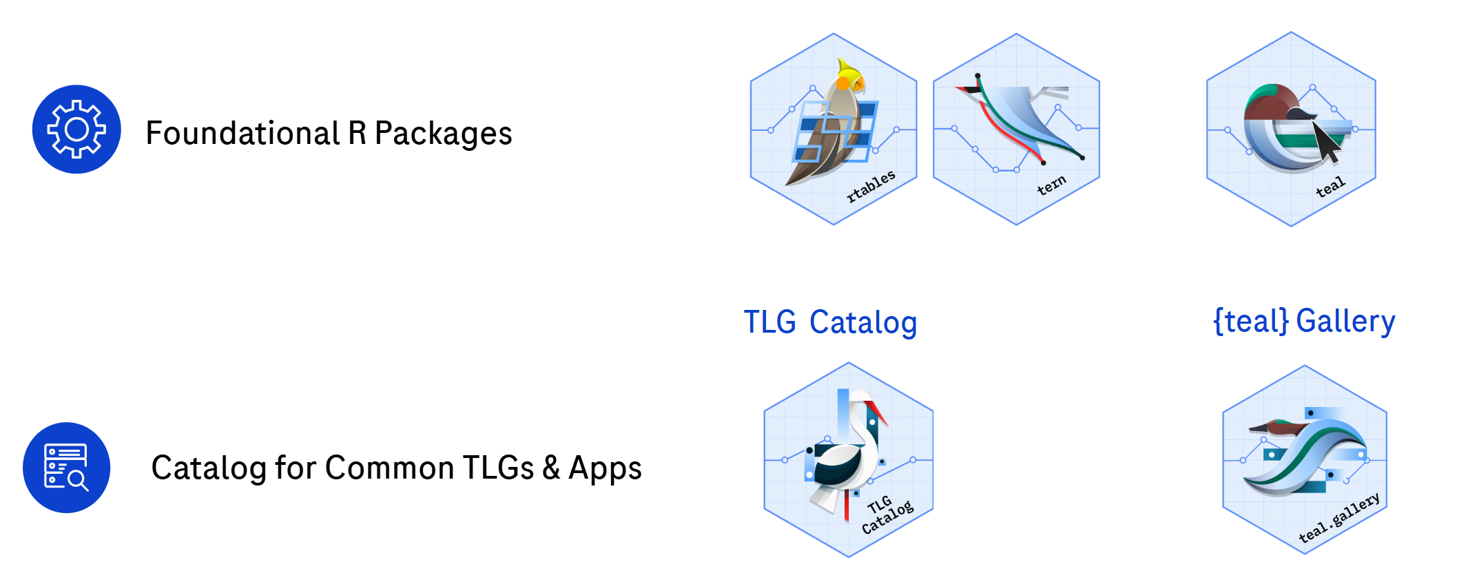
Accelerating Clinical Reporting

A collection of open-sourced R packages, which enables fast and efficient insights generation under clinical research settings, for both exploratory and regulatory purposes.
Working towards a complete solution for R-based insights delivery
From an humble data.frame to mesmerizing interactive tables!
Recommended: Enter the dedicated RStudio Cloud work space (with packages pre-installed) to complete Exercise 1. It may still be helpful to peek at the exercises web page to verify that your results match the desired output.
→ R in Pharma RStudio Cloud work space ←
Otherwise: Use your personal computer and follow along the exercises on the website. Challenge yourself not to peek at the code solutions until you have completed the exercise.
Create a demographic table by using only {dplyr}.
10:00
# Load necessary libraries
library(dplyr)

# Sample data frame with demographic data
set.seed(123)
data <- data.frame(
  id = 1:100,
  age = sample(18:80, 100, replace = TRUE),
  gender = sample(c("Male", "Female"), 100, replace = TRUE),
  treatment = sample(c("Treatment A", "Treatment B"), 100, replace = TRUE)
)

head(data)| id | age | gender | treatment |
|---|---|---|---|
| 1 | 48 | Female | Treatment B |
| 2 | 32 | Female | Treatment B |
| 3 | 68 | Male | Treatment A |
| 4 | 31 | Female | Treatment B |
| 5 | 20 | Female | Treatment B |
| 6 | 59 | Male | Treatment B |
# Count participants per treatment group to get labels with counts
treatment_counts <- data |>
  count(treatment) |>
  mutate(treatment_label = paste0(treatment, " (N=", n, ")"))

# Create the demographic summary table
demographic_table <- data |>
  # Join with treatment counts to include the labeled treatment names
  left_join(treatment_counts, by = "treatment") |>
  # Summarize age, female, and male counts and percentages by the labeled treatment
  group_by(treatment_label) |>
  summarise(
    `Mean Age (SD)` = paste0(round(mean(age), 1), " (", round(sd(age), 1), ")"),
    `N Female (%)` = paste0(sum(gender == "Female"), " (", round(sum(gender == "Female") / n() * 100, 1), "%)"),
    `N Male (%)` = paste0(sum(gender == "Male"), " (", round(sum(gender == "Male") / n() * 100, 1), "%)"),
    .groups = "drop"
  ) |>
  # Transpose for easy review if needed
  t() |>
print()| Treatment A (N=51) | Treatment B (N=49) | |
|---|---|---|
| Mean Age (SD) | 50.3 (17.9) | 45.7 (16.3) |
| N Female (%) | 27 (52.9%) | 28 (57.1%) |
| N Male (%) | 24 (47.1%) | 21 (42.9%) |
Here is how to do it in {rtables} (for tabulation) and {tern} (for the summary functions):
| Treatment B | Treatment A | |
|---|---|---|
| gender | ||
| n | 49 | 51 |
| Female | 28 (57.1%) | 27 (52.9%) |
| Male | 21 (42.9%) | 24 (47.1%) |
| age | ||
| n | 49 | 51 |
| Mean (SD) | 45.7 (16.3) | 50.3 (17.9) |
| Median | 44.0 | 49.0 |
| Min - Max | 20.0 - 79.0 | 21.0 - 80.0 |
Check {rtables} documentation
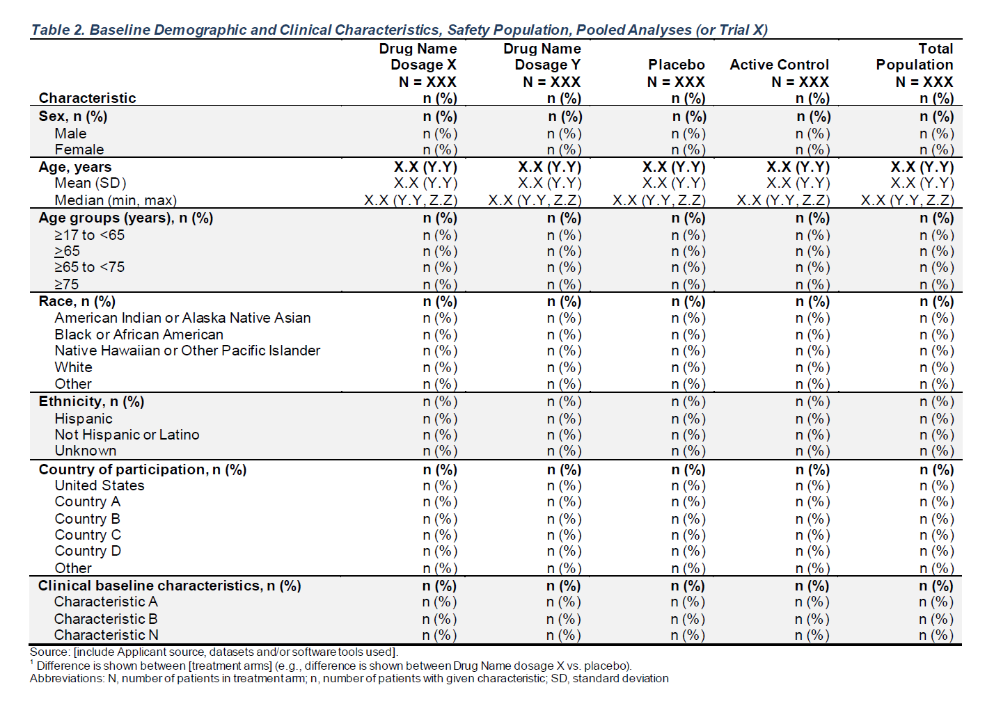
Build the following demographic table using {rtables} or {gtsummary}.


Check cardinal
Data Tip
Checking {cardinal} template you can directly use the synthetic data set as described.
adsl <- random.cdisc.data::cadsl
advs <- random.cdisc.data::cadvs
# Pre-Processing - Add any variables needed in your table to df
adsl <- adsl |>
mutate(AGEGR1 = as.factor(case_when(
AGE >= 17 & AGE < 65 ~ "≥17 to <65",
AGE >= 65 ~ "≥65",
AGE >= 65 & AGE < 75 ~ "≥65 to <75",
AGE >= 75 ~ "≥75"
)))
advs <- advs |>
filter(AVISIT == "BASELINE", VSTESTCD == "TEMP") |>
select("USUBJID", "AVAL")
anl <- left_join(adsl, advs, by = "USUBJID")
head(anl)| Study Identifier | Unique Subject Identifier | Subject Identifier for the Study | Study Site Identifier | Age | Age Units | Sex | Race | Ethnicity | Country | Subject Death Flag | Investigator Identifier | Investigator Name | Description of Planned Arm | Planned Arm Code | Description of Actual Arm | Actual Arm Code | Planned Treatment for Period 01 | Actual Treatment for Period 01 | Planned Treatment for Period 02 | Actual Treatment for Period 02 | Geographic Region 1 | Stratification Factor 1 | Stratification Factor 2 | Continuous Level Biomarker 1 | Categorical Level Biomarker 2 | Intent-To-Treat Population Flag | Safety Population Flag | Response Evaluable Population Flag | Biomarker Evaluable Population Flag | AE Leading to Drug Withdrawal Flag | Date of Randomization | Datetime of First Exposure to Treatment | Datetime of Last Exposure to Treatment | Datetime of First Exposure to Treatment in Period 01 | Datetime of Last Exposure in Period 01 | Datetime of First Exposure to Treatment in Period 02 | Datetime of Last Exposure to Treatment in Period 02 | Period 01 Start Datetime | Period 01 End Datetime | Period 02 Start Datetime | Period 02 End Datetime | End of Study Status | End of Treatment Status | End of Study Date | End of Study Relative Day | Reason for Discontinuation from Study | Date of Death | Cause of Death | Cause of Death Category | Elapsed Days from Last Dose to Death | Last Dose to Death - Days Elapsed Grp 1 | Date Last Known Alive | Relative Day of Death | Autopsy Performed | AGEGR1 | Analysis Value |
|---|---|---|---|---|---|---|---|---|---|---|---|---|---|---|---|---|---|---|---|---|---|---|---|---|---|---|---|---|---|---|---|---|---|---|---|---|---|---|---|---|---|---|---|---|---|---|---|---|---|---|---|---|---|---|---|---|
| AB12345 | AB12345-CHN-3-id-128 | id-128 | CHN-3 | 32 | YEARS | M | ASIAN | HISPANIC OR LATINO | CHN | Y | INV ID CHN-3 | Dr. CHN-3 Doe | A: Drug X | ARM A | A: Drug X | ARM A | A: Drug X | A: Drug X | B: Placebo | A: Drug X | Asia | C | S2 | 14.424934 | MEDIUM | Y | Y | Y | Y | N | 2019-02-22 | 2019-02-24 11:09:25.683 | 2022-02-12 04:28:08.683 | 2019-02-24 11:09:25.683 | 2021-02-11 22:28:08.683 | 2021-02-11 22:28:08.683 | 2022-02-12 04:28:08.683 | 2019-02-24 11:09:25.683 | 2021-02-11 22:28:08.683 | 2021-02-11 22:28:08.683 | 2022-02-12 04:28:08.683 | DISCONTINUED | DISCONTINUED | 2022-02-12 | 1084 | DEATH | 2022-03-06 | ADVERSE EVENT | ADVERSE EVENT | 22 | <=30 | 2022-03-06 | 1105 | Yes | ≥17 to <65 | 37.21088 |
| AB12345 | AB12345-CHN-15-id-262 | id-262 | CHN-15 | 35 | YEARS | M | BLACK OR AFRICAN AMERICAN | NOT HISPANIC OR LATINO | CHN | N | INV ID CHN-15 | Dr. CHN-15 Doe | C: Combination | ARM C | C: Combination | ARM C | C: Combination | C: Combination | B: Placebo | C: Combination | Asia | C | S1 | 4.055463 | LOW | Y | Y | N | N | Y | 2019-02-26 | 2019-02-26 09:05:10.683 | 2022-02-26 03:05:10.683 | 2019-02-26 09:05:10.683 | 2021-02-25 21:05:10.683 | 2021-02-25 21:05:10.683 | 2022-02-26 03:05:10.683 | 2019-02-26 09:05:10.683 | 2021-02-25 21:05:10.683 | 2021-02-25 21:05:10.683 | 2022-02-26 03:05:10.683 | COMPLETED | COMPLETED | 2022-02-26 | 1096 | NA | NA | NA | NA | NA | NA | 2022-03-17 | NA | NA | ≥17 to <65 | 37.91017 |
| AB12345 | AB12345-RUS-3-id-378 | id-378 | RUS-3 | 30 | YEARS | F | ASIAN | NOT HISPANIC OR LATINO | RUS | N | INV ID RUS-3 | Dr. RUS-3 Doe | C: Combination | ARM C | C: Combination | ARM C | C: Combination | C: Combination | A: Drug X | B: Placebo | Eurasia | A | S1 | 2.803240 | HIGH | Y | Y | Y | N | N | 2019-02-24 | 2019-02-28 03:19:22.683 | 2022-02-27 21:19:22.683 | 2019-02-28 03:19:22.683 | 2021-02-27 15:19:22.683 | 2021-02-27 15:19:22.683 | 2022-02-27 21:19:22.683 | 2019-02-28 03:19:22.683 | 2021-02-27 15:19:22.683 | 2021-02-27 15:19:22.683 | 2022-02-27 21:19:22.683 | COMPLETED | COMPLETED | 2022-02-27 | 1096 | NA | NA | NA | NA | NA | NA | 2022-03-11 | NA | NA | ≥17 to <65 | 35.53659 |
| AB12345 | AB12345-CHN-11-id-220 | id-220 | CHN-11 | 26 | YEARS | F | ASIAN | NOT HISPANIC OR LATINO | CHN | N | INV ID CHN-11 | Dr. CHN-11 Doe | B: Placebo | ARM B | B: Placebo | ARM B | B: Placebo | B: Placebo | B: Placebo | B: Placebo | Asia | B | S2 | 10.262734 | MEDIUM | Y | Y | Y | Y | N | 2019-02-27 | 2019-03-01 13:33:19.683 | 2022-03-01 07:33:19.683 | 2019-03-01 13:33:19.683 | 2021-03-01 01:33:19.683 | 2021-03-01 01:33:19.683 | 2022-03-01 07:33:19.683 | 2019-03-01 13:33:19.683 | 2021-03-01 01:33:19.683 | 2021-03-01 01:33:19.683 | 2022-03-01 07:33:19.683 | COMPLETED | COMPLETED | 2022-03-01 | 1096 | NA | NA | NA | NA | NA | NA | 2022-03-26 | NA | NA | ≥17 to <65 | 37.75094 |
| AB12345 | AB12345-CHN-7-id-267 | id-267 | CHN-7 | 40 | YEARS | M | ASIAN | NOT HISPANIC OR LATINO | CHN | N | INV ID CHN-7 | Dr. CHN-7 Doe | B: Placebo | ARM B | B: Placebo | ARM B | B: Placebo | B: Placebo | C: Combination | A: Drug X | Asia | C | S1 | 6.206763 | LOW | Y | Y | N | N | N | 2019-03-01 | 2019-03-02 00:09:33.683 | 2022-03-01 18:09:33.683 | 2019-03-02 00:09:33.683 | 2021-03-01 12:09:33.683 | 2021-03-01 12:09:33.683 | 2022-03-01 18:09:33.683 | 2019-03-02 00:09:33.683 | 2021-03-01 12:09:33.683 | 2021-03-01 12:09:33.683 | 2022-03-01 18:09:33.683 | COMPLETED | COMPLETED | 2022-03-01 | 1096 | NA | NA | NA | NA | NA | NA | 2022-03-15 | NA | NA | ≥17 to <65 | 33.65185 |
| AB12345 | AB12345-CHN-15-id-201 | id-201 | CHN-15 | 49 | YEARS | M | ASIAN | NOT HISPANIC OR LATINO | CHN | Y | INV ID CHN-15 | Dr. CHN-15 Doe | C: Combination | ARM C | C: Combination | ARM C | C: Combination | C: Combination | B: Placebo | C: Combination | Asia | C | S2 | 6.906799 | MEDIUM | Y | Y | Y | N | N | 2019-03-05 | 2019-03-05 15:24:07.683 | 2022-02-19 04:06:48.683 | 2019-03-05 15:24:07.683 | 2021-02-18 22:06:48.683 | 2021-02-18 22:06:48.683 | 2022-02-19 04:06:48.683 | 2019-03-05 15:24:07.683 | 2021-02-18 22:06:48.683 | 2021-02-18 22:06:48.683 | 2022-02-19 04:06:48.683 | DISCONTINUED | DISCONTINUED | 2022-02-19 | 1082 | DEATH | 2022-02-22 | ADVERSE EVENT | ADVERSE EVENT | 3 | <=30 | 2022-02-22 | 1084 | Yes | ≥17 to <65 | 36.49592 |
Tip
Check the function make_table_02 or make_table_02_gtsum from {cardinal} here
15:00
df <- anl |>
  df_explicit_na()

vars <- c("SEX", "AGE", "AGEGR1", "RACE", "ETHNIC", "COUNTRY")
lbl_vars <- formatters::var_labels(df, fill = TRUE)[vars]

lyt <- basic_table(show_colcounts = TRUE) |>
  split_cols_by("ARM", split_fun = add_overall_level("Total Population", first = FALSE)) |>
  analyze_vars(
    vars = vars,
    var_labels = lbl_vars,
    show_labels = "visible",
    .stats = c("mean_sd", "median_range", "count_fraction"),
    .formats = NULL,
    na.rm = FALSE
  ) |>
  append_topleft("Characteristic")

tbl <- build_table(lyt, df = df) |>
  prune_table()

tbl
Characteristic | A: Drug X (N=134) | B: Placebo (N=134) | C: Combination (N=132) | Total Population (N=400) |
|---|---|---|---|---|
Sex |
|
|
|
|
F | 79 (59%) | 82 (61.2%) | 70 (53%) | 231 (57.8%) |
M | 55 (41%) | 52 (38.8%) | 62 (47%) | 169 (42.2%) |
Age |
|
|
|
|
Mean (SD) | 33.8 (6.6) | 35.4 (7.9) | 35.4 (7.7) | 34.9 (7.4) |
Median (Min - Max) | 33.0 (21.0 - 50.0) | 35.0 (21.0 - 62.0) | 35.0 (20.0 - 69.0) | 34.0 (20.0 - 69.0) |
AGEGR1 |
|
|
|
|
≥17 to <65 | 134 (100%) | 134 (100%) | 131 (99.2%) | 399 (99.8%) |
≥65 | 0 | 0 | 1 (0.8%) | 1 (0.2%) |
Race |
|
|
|
|
ASIAN | 68 (50.7%) | 67 (50%) | 73 (55.3%) | 208 (52%) |
BLACK OR AFRICAN AMERICAN | 31 (23.1%) | 28 (20.9%) | 32 (24.2%) | 91 (22.8%) |
WHITE | 27 (20.1%) | 26 (19.4%) | 21 (15.9%) | 74 (18.5%) |
AMERICAN INDIAN OR ALASKA NATIVE | 8 (6%) | 11 (8.2%) | 6 (4.5%) | 25 (6.2%) |
MULTIPLE | 0 | 1 (0.7%) | 0 | 1 (0.2%) |
NATIVE HAWAIIAN OR OTHER PACIFIC ISLANDER | 0 | 1 (0.7%) | 0 | 1 (0.2%) |
Ethnicity |
|
|
|
|
HISPANIC OR LATINO | 15 (11.2%) | 18 (13.4%) | 15 (11.4%) | 48 (12%) |
NOT HISPANIC OR LATINO | 104 (77.6%) | 103 (76.9%) | 101 (76.5%) | 308 (77%) |
NOT REPORTED | 6 (4.5%) | 10 (7.5%) | 11 (8.3%) | 27 (6.8%) |
UNKNOWN | 9 (6.7%) | 3 (2.2%) | 5 (3.8%) | 17 (4.2%) |
Country |
|
|
|
|
CHN | 74 (55.2%) | 81 (60.4%) | 64 (48.5%) | 219 (54.8%) |
USA | 10 (7.5%) | 13 (9.7%) | 17 (12.9%) | 40 (10%) |
BRA | 13 (9.7%) | 7 (5.2%) | 10 (7.6%) | 30 (7.5%) |
PAK | 12 (9%) | 9 (6.7%) | 10 (7.6%) | 31 (7.8%) |
NGA | 8 (6%) | 7 (5.2%) | 11 (8.3%) | 26 (6.5%) |
RUS | 5 (3.7%) | 8 (6%) | 6 (4.5%) | 19 (4.8%) |
JPN | 5 (3.7%) | 4 (3%) | 9 (6.8%) | 18 (4.5%) |
GBR | 4 (3%) | 3 (2.2%) | 2 (1.5%) | 9 (2.2%) |
CAN | 3 (2.2%) | 2 (1.5%) | 3 (2.3%) | 8 (2%) |
library(gtsummary)

df <- df |> df_explicit_na()
vars <- c("SEX", "AGE", "AGEGR1", "RACE", "ETHNIC", "COUNTRY")
lbl_vars <- formatters::var_labels(df, fill = TRUE)[vars]

tbl <- df  |>
  select(c(vars, "ARM")) |>
  tbl_summary(
    by = "ARM",
    type = all_continuous() ~ "continuous2",
    statistic = list(
      all_continuous() ~ c(
        "{mean} ({sd})",
        "{median} ({min} - {max})"
      ),
      all_categorical() ~ "{n} ({p}%)"
    ),
    digits = all_continuous() ~ 1,
    missing = "ifany",
    label = as.list(lbl_vars) |> setNames(vars)
  ) |>
  gtsummary::bold_labels() |>
  modify_header(all_stat_cols() ~ "**{level}**  \nN = {n}") |>
  add_overall(last = TRUE, col_label = paste0("**", "Total Population", "**  \nN = {n}")) |>
  gtsummary::add_stat_label(label = all_continuous2() ~ c("Mean (SD)", "Median (min - max)")) |>
  modify_footnote(update = everything() ~ NA) |>
  gtsummary::modify_column_alignment(columns = all_stat_cols(), align = "right")

tbl| Characteristic | A: Drug X N = 134 |
B: Placebo N = 134 |
C: Combination N = 132 |
Total Population N = 400 |
|---|---|---|---|---|
| Sex, n (%) | ||||
| F | 79 (59%) | 82 (61%) | 70 (53%) | 231 (58%) |
| M | 55 (41%) | 52 (39%) | 62 (47%) | 169 (42%) |
| Age | ||||
| Mean (SD) | 33.8 (6.6) | 35.4 (7.9) | 35.4 (7.7) | 34.9 (7.4) |
| Median (min - max) | 33.0 (21.0 - 50.0) | 35.0 (21.0 - 62.0) | 35.0 (20.0 - 69.0) | 34.0 (20.0 - 69.0) |
| AGEGR1, n (%) | ||||
| ≥17 to <65 | 134 (100%) | 134 (100%) | 131 (99%) | 399 (100%) |
| ≥65 | 0 (0%) | 0 (0%) | 1 (0.8%) | 1 (0.3%) |
| Race, n (%) | ||||
| ASIAN | 68 (51%) | 67 (50%) | 73 (55%) | 208 (52%) |
| BLACK OR AFRICAN AMERICAN | 31 (23%) | 28 (21%) | 32 (24%) | 91 (23%) |
| WHITE | 27 (20%) | 26 (19%) | 21 (16%) | 74 (19%) |
| AMERICAN INDIAN OR ALASKA NATIVE | 8 (6.0%) | 11 (8.2%) | 6 (4.5%) | 25 (6.3%) |
| MULTIPLE | 0 (0%) | 1 (0.7%) | 0 (0%) | 1 (0.3%) |
| NATIVE HAWAIIAN OR OTHER PACIFIC ISLANDER | 0 (0%) | 1 (0.7%) | 0 (0%) | 1 (0.3%) |
| OTHER | 0 (0%) | 0 (0%) | 0 (0%) | 0 (0%) |
| UNKNOWN | 0 (0%) | 0 (0%) | 0 (0%) | 0 (0%) |
| Ethnicity, n (%) | ||||
| HISPANIC OR LATINO | 15 (11%) | 18 (13%) | 15 (11%) | 48 (12%) |
| NOT HISPANIC OR LATINO | 104 (78%) | 103 (77%) | 101 (77%) | 308 (77%) |
| NOT REPORTED | 6 (4.5%) | 10 (7.5%) | 11 (8.3%) | 27 (6.8%) |
| UNKNOWN | 9 (6.7%) | 3 (2.2%) | 5 (3.8%) | 17 (4.3%) |
| Country, n (%) | ||||
| CHN | 74 (55%) | 81 (60%) | 64 (48%) | 219 (55%) |
| USA | 10 (7.5%) | 13 (9.7%) | 17 (13%) | 40 (10%) |
| BRA | 13 (9.7%) | 7 (5.2%) | 10 (7.6%) | 30 (7.5%) |
| PAK | 12 (9.0%) | 9 (6.7%) | 10 (7.6%) | 31 (7.8%) |
| NGA | 8 (6.0%) | 7 (5.2%) | 11 (8.3%) | 26 (6.5%) |
| RUS | 5 (3.7%) | 8 (6.0%) | 6 (4.5%) | 19 (4.8%) |
| JPN | 5 (3.7%) | 4 (3.0%) | 9 (6.8%) | 18 (4.5%) |
| GBR | 4 (3.0%) | 3 (2.2%) | 2 (1.5%) | 9 (2.3%) |
| CAN | 3 (2.2%) | 2 (1.5%) | 3 (2.3%) | 8 (2.0%) |
| CHE | 0 (0%) | 0 (0%) | 0 (0%) | 0 (0%) |
Lets try now to build an ANCOVA efficacy table with a single visit and single endpoint.
Tip
Peak at solution AOVT02 on the TLG-catalog and try to understand each function!!
10:00
Check TLG-catalog for hundreds of ready-made TLGs
Lets try now to use the above table to build a {teal} interactive table!
Tip
Peak at solution AOVT02 for teal too! and try to understand each function!!
10:00
Check TLG-catalog for hundreds of ready-made TLGs
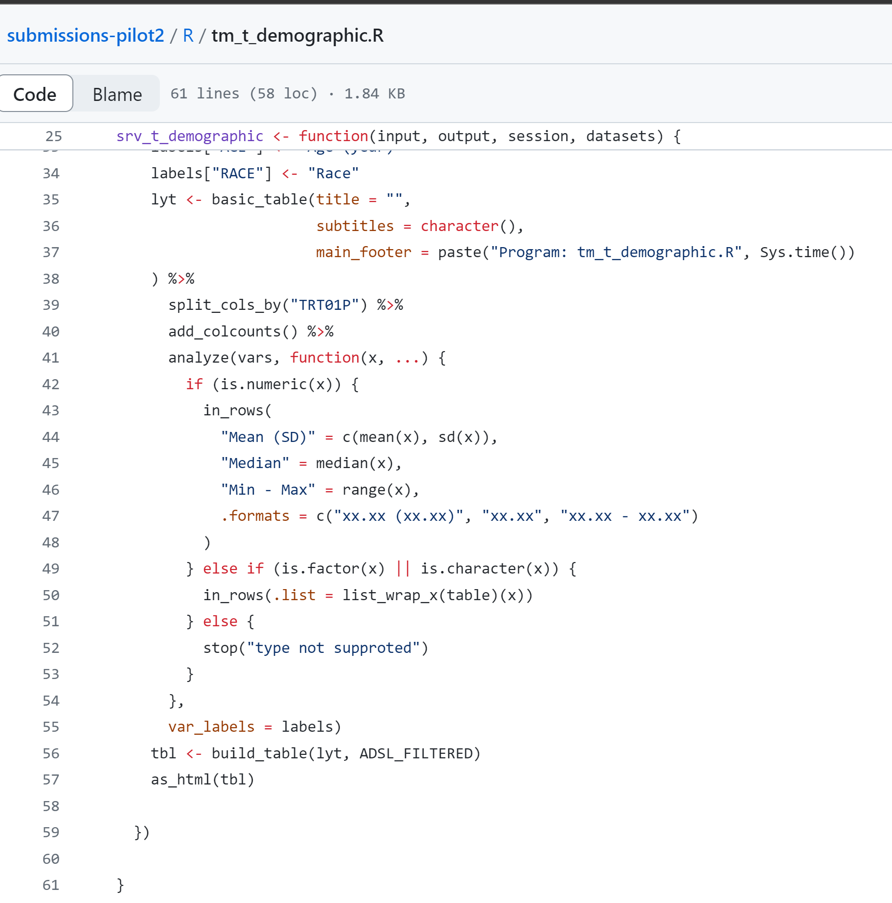
Try to use the data from before (Exercise 1) to make your own teal app (tip: use tm_t_summary).
Lets try now to create an efficacy Kaplan-Meier plot.
Tip
Peak at solution KMG01 and try to understand each function!!
10:00
Check TLG-catalog for hundreds of ready-made TLGs
Play with efficacy app ;)
Short-Term Considerations:
The migration process requires initial investment in terms of time, resources, and training. Existing workflows and scripts need to be rewritten or adapted, which can be a significant effort.
Long-Term Benefits:
The long-term benefits of migrating to R include cost savings, increased flexibility, access to a broader talent pool, and staying ahead in terms of technological advancements. If regulatory bodies continue to increase acceptance of R, the case for migration becomes even stronger.
Where to find more on NEST
Where to find more on NEST
Where to find more on NEST
How can I get involved?
Notice a 🐛 or an idea for enhancements💡?
We encourage you to collaborate with us and contribute our code base can be found here: https://github.com/insightsengineering
🖮 You can get in touch with us on slack #pharmaverse-pkgs channel here
📧 or contact Leena our product owner if you are interested in industry collaboration (leena.khatri@roche.com)
🙏 Click here to submit workshop feedback